WWW'26 | SS-MoE:显存墙下的 MoE 推理,Self-Speculative Decoding 怎么救场?
WWW’26 | SS-MoE:显存墙下的 MoE 推理,Self-Speculative Decoding 怎么救场?
原文:Self-Speculative Decoding for On-device MoE Acceleration ACM WWW 2026
这是 Self-Speculative Decoding 系列第四篇。前三篇(Draft & Verify、LayerSkip、SWIFT)讲的都是 Dense 模型上的 Self-SD。这一篇换了个赛道:MoE 架构,而且是专门针对端侧显存受限场景的。
1. MoE 推理的核心矛盾
先交代下背景。
MoE 火是真的火——DeepSeek、Qwen3-MoE、Mixtral,主流 LLM 里 MoE 越来越多。吸引力很直接:总参数量大,但每次推理只激活 top-k 个 expert(Sparse Activation),计算量远小于同量级 Dense 模型。
但实际跑下来,端侧部署有个结结实实的坑:
下图是 MoE 模型参数的组成——总参数里 89.9% 是 expert 参数;激活参数里,expert 也占了 45.5%:
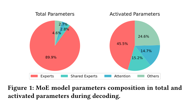
问题来了:虽然每次推理只用 top-k 个 expert,但所有 expert 的参数都得加载进显存。一台显存受限的 GPU 根本装不下,于是得做 CPU offloading——把 expert 参数放在 CPU 内存,推理时按需搬过来。
但 CPU offloading 带来了新麻烦:下一层 router 选哪个 expert,在当前层算完之前是未知的,预取只能猜,猜错了就得等 IO 延迟,latency 暴增。
稀疏激活节省计算、全量加载消耗显存、CPU offloading 引入 IO 瓶颈——这是整个 MoE 端侧推理领域的核心矛盾。SS-MoE 把 Self-Speculative Decoding 引进来,从算法层面提供了一个新出口。
2. 关键洞察:少激活几个 expert,质量掉多少?
SS-MoE 的出发点是一个实验性观察:
下图 (a) 展示了在 DeepSeek 模型上,随着每个 token 激活的 expert 数量从 1 减少到 6,ARC-Easy 精度(蓝线)和 TPS(粉线)的变化:
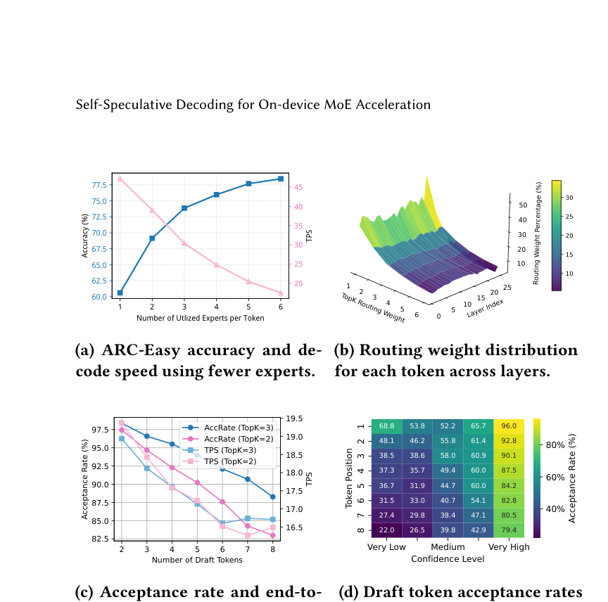
精度随 expert 数量单调提升,但用 top-3 expert 就能达到 top-6 的 94% 精度(约 72% vs 78%),同时速度提升明显。图 (b) 是各层 routing 权重分布——top-2 的权重占了累计分布的 60% 以上,说明少数 expert 承担了大部分贡献。
图 (c) 进一步说明:draft token 的 acceptance rate 随 draft 长度增加而略降,但始终保持在 85% 以上(TopK=3 时)。图 (d) 则直接说明了 confidence 感知的合理性:高置信度位置的 acceptance rate 高达 96%,低置信度位置也有 52%-68%。
这就是 SS-MoE 的核心 insight:用少量 routed expert 生成草稿,大概率能被完整模型接受,而且草稿阶段的 IO 开销更小,prefetch 更准。
3. 方法:SS-MoE 的三个组件
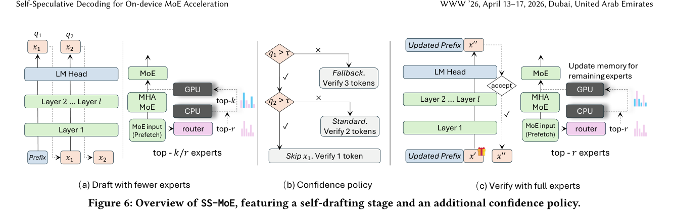
下图是 SS-MoE 的整体架构,分三部分:(a) draft 阶段用更少 expert,(b) 置信度策略,(c) verify 阶段用完整 expert:
3.1 MoE 前向传播:先搞清楚正常情况下发生了什么
一个标准的 MoE 层的前向传播分三步:
def moe_layer_forward(x, router, experts, k=2):
    """
    x: [seq_len, hidden_dim]
    router: 线性层,输出每个 token 对所有 expert 的得分
    experts: N 个 FFN expert
    k: 每个 token 激活的 expert 数量
    """
    # Step 1: router 给每个 token 打分
    router_scores = softmax(router(x))  # [seq_len, N_experts]

    # Step 2: 每个 token 选 top-k 个 expert
    top_k_indices = topk(router_scores, k)     # [seq_len, k]
    top_k_weights  = gather(router_scores, top_k_indices)  # [seq_len, k]

    # Step 3: 被选中的 expert 计算输出,加权求和
    output = zeros_like(x)
    for i, idx in enumerate(top_k_indices):
        for j, expert_id in enumerate(idx):
            output[i] += top_k_weights[i][j] * experts[expert_id](x[i])

    return output
问题在 Step 3:experts[expert_id] 这一步需要 expert 参数在 GPU 上。如果 GPU 显存不够存所有 N 个 expert,就得从 CPU 临时搬。而 expert_id 只有跑完 Step 1 和 Step 2 才能知道——所以无法提前准备,只能串行等 IO。
3.2 SS-MoE 的 Draft-Verify 流程
SS-MoE 把 MoE 推理改成 Draft + Verify 两阶段。核心是:draft 阶段每层只用 top-r 个 expert(r < k),verify 阶段用完整的 top-k 个 expert。
def ss_moe_draft(x, router, expert_cache, r=1):
    """
    Draft 阶段:每层只用 top-r 个 expert
    r < k,速度快,IO 少,但输出质量略低
    """
    router_scores = softmax(router(x))
    top_r_indices = topk(router_scores, r)   # 只选 r 个,而非 k 个
    top_r_weights  = gather(router_scores, top_r_indices)

    # 关键:top-r 的 expert 是 top-k 的子集
    # 这些 expert 大概率已经在 GPU 的 expert_cache 里(热 expert)
    output = zeros_like(x)
    for i, idx in enumerate(top_r_indices):
        for j, expert_id in enumerate(idx):
            expert = expert_cache.get(expert_id)  # 命中缓存,无 IO 等待
            output[i] += top_r_weights[i][j] * expert(x[i])

    return output, router_scores  # 保存 router_scores 供 verify 用

def ss_moe_verify(x_full, router_scores_draft, expert_cache, k=2):
    """
    Verify 阶段:用完整 top-k 个 expert 并行验证所有 draft token
    额外加载 draft 阶段未使用的 (k-r) 个 expert
    """
    top_k_indices = topk(router_scores_draft, k)
    # 只需加载 top_k 中不在 top_r 里的那部分 expert(增量加载)
    new_experts_needed = top_k_indices[r:]
    expert_cache.prefetch(new_experts_needed)

    # 正常 top-k 前向传播
    return moe_layer_forward(x_full, router_scores_draft, expert_cache, k)
这里有个非常优雅的设计:draft 用的 top-r expert 是 verify 用的 top-k expert 的子集。所以 verify 阶段不需要重新加载 draft 已经用过的 expert,只需要增量加载剩余的 (k-r) 个 expert,IO 开销大幅减少。
3.3 Expert Cache + 预取优化
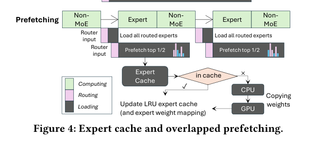
SS-MoE 把 GPU 显存当成 expert 的 LRU cache 管理。下图展示了预取(prefetching)的设计:
Expert Cache 策略:
class ExpertCache:
    def __init__(self, capacity):
        # GPU 显存只能容纳 capacity 个 expert
        self.cache = LRU_dict(capacity)

    def get(self, expert_id):
        if expert_id in self.cache:
            return self.cache[expert_id]  # 缓存命中,直接返回
        else:
            # 缓存未命中:从 CPU 加载(同步,有延迟)
            expert = cpu_memory.load(expert_id)
            self.cache[expert_id] = expert  # LRU 淘汰最久未用的
            return expert

    def async_prefetch(self, expert_ids):
        # 异步预取:启动 CPU→GPU 传输,不阻塞当前计算
        for eid in expert_ids:
            if eid not in self.cache:
                launch_async_transfer(cpu_memory[eid], target=gpu_buffer)
Overlapped Prefetch(计算与 IO 重叠):
draft 阶段只用 top-r 个 expert,比 top-k 少激活了 (k-r) 个 expert。这些”省下来”的 IO 带宽可以用来提前预取下一层的 expert:
时间轴:
  Layer l compute  : [==== draft top-r expert 计算 ====]
  Layer l+1 prefetch:     [-- 异步加载 layer l+1 的 top-r expert --]
                    ↑
                 重叠区域越大,IO 延迟被计算时间掩盖的越多
由于 draft 阶段激活的 expert 少,router 输出更快确定,预取启动时间更早,命中率更高。这是 draft 用少 expert 带来的系统级收益,不只是计算量的节省。
3.4 完整算法:Draft + Verify 循环
下面是 SS-MoE 的完整推理伪代码(Algorithm 1):
def ss_moe_inference(prompt, model, expert_cache,
                     r=1, k=2, max_draft=5, τ=0.5, T=0):
    """
    r: draft 阶段每层激活的 routed expert 数
    k: verify 阶段每层激活的 routed expert 数(k > r)
    max_draft: 最大 draft token 数
    τ: 置信度阈值
    T: 温度(T=0 为 conservative 模式)
    """
    context = prompt
    output = []

    while not done:
        # ─── Draft 阶段 ────────────────────────────────────────
        draft_tokens = []
        draft_probs = []

        for j in range(max_draft):
            # 每个 MoE 层只用 top-r expert
            hidden = context + draft_tokens
            for layer in model.layers:
                if layer.is_moe:
                    hidden, router_scores = ss_moe_draft(hidden, layer.router,
                                                          expert_cache, r=r)
                    # 同时预取下一层的 expert(计算 IO 重叠)
                    expert_cache.async_prefetch(predict_next_layer_experts(hidden))
                else:
                    hidden = layer(hidden)

            probs = softmax(model.lm_head(hidden[-1]))
            conf = probs.max()
            draft_tokens.append(probs.argmax())
            draft_probs.append(probs)

            # 置信度低 → 提前停止
            if conf < τ:
                break

        # ─── Verify 阶段 ──────────────────────────────────────
        # 一次 batch forward,并行验证所有 draft token
        # 每个 MoE 层用完整 top-k expert
        verify_context = context + draft_tokens
        verify_probs = full_model_forward(verify_context, expert_cache, k=k)
        # verify_probs[i] 是完整模型对位置 i 的输出概率分布

        # ─── 接受/拒绝 ────────────────────────────────────────
        accepted = []
        for j, (d_t, q_t, p_t) in enumerate(
                zip(draft_tokens, draft_probs, verify_probs)):

            if T == 0:
                # Conservative 模式:严格无损,标准接受条件
                accept_prob = min(1.0, p_t[d_t] / q_t[d_t])
                if random() < accept_prob:
                    accepted.append(d_t)
                else:
                    # 拒绝:从修正分布采样,然后截断
                    correction = sample(norm(max(0, p_t - q_t)))
                    accepted.append(correction)
                    break
            else:
                # Adaptive 模式:高置信度的 draft token 宽松接受
                # 允许少量近似误差换取更高 TPS
                if q_t[d_t] > τ and p_t[d_t] / q_t[d_t] > (1 - T):
                    accepted.append(d_t)
                else:
                    accepted.append(sample(p_t))
                    break

        output.extend(accepted)
        context = context + accepted

    return output
3.5 置信度感知的自适应验证
两种模式对应不同的精度-速度权衡:
- Conservative(T=0):严格遵循推测解码的无损条件
min(1, p/q),输出分布与完整自回归完全一致,精度不低于 4-bit 量化基线 - Adaptive(T>0):允许接受置信度高但严格来说有偏差的 draft token,用极小的精度损失换取显著更高的 TPS。论文报告自适应模式下精度损失”nearly lossless”
4. 实验结果
测试模型:DeepSeek MoE 系列 和 Moonlight MoE,任务覆盖 MT-Bench、Translation、Summarization、QA、Math、RAG、Code,显存受限 GPU 环境。
主要结果如下表:
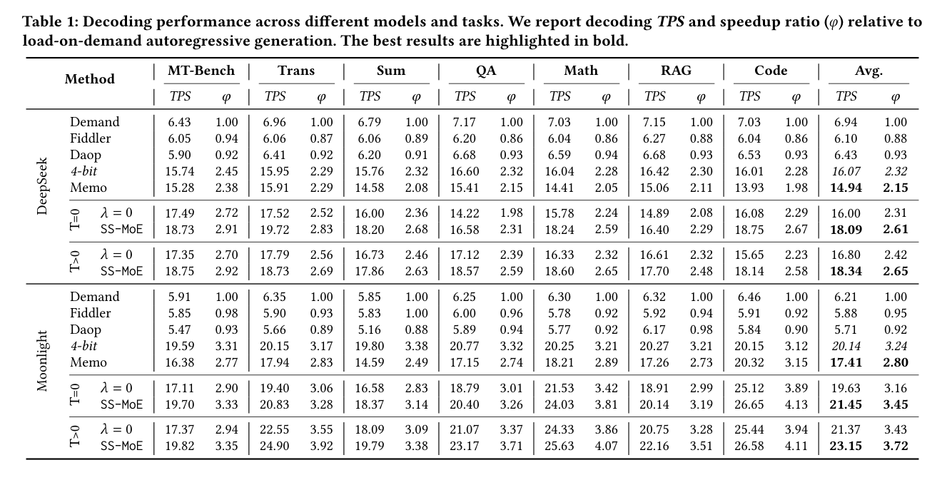
几个关键数字:
- DeepSeek + SS-MoE(T>0):平均 TPS 18.34,加速比 2.65×(vs. load-on-demand 基线)
- Moonlight + SS-MoE(T>0):平均 TPS 23.15,加速比 3.72×
- 对比 4-bit 量化(2.32×/3.24×):SS-MoE 在保持更高精度的同时,加速比明显更高
不同显存 budget 下的表现:
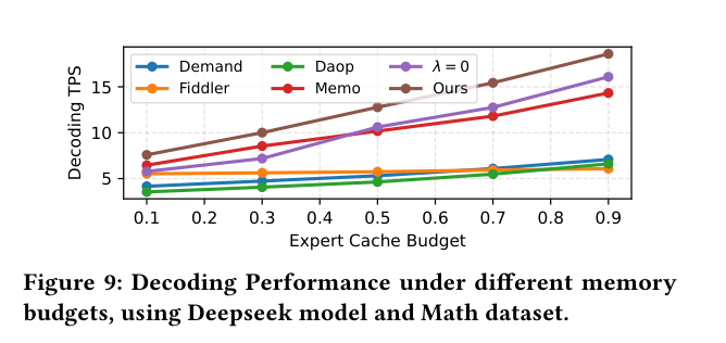
即使 cache budget 很小(0.1),SS-MoE(Ours,棕线)也显著高于所有 baseline。随着 cache budget 增大,优势持续扩大。
5. 这篇工作在系列里的位置
前三篇 Self-SD 工作”跳”的是 Transformer 的中间层。SS-MoE 把这个逻辑迁移到 MoE,”跳”的是每层里的部分 expert。
SS-MoE 带来了三重收益:
- 计算量减少:draft 阶段 FLOPs 降低(少激活 expert)
- IO 开销降低:draft 阶段需要从 CPU 加载的 expert 更少
- Prefetch 命中率提升:更早确定 router 结果 → 更早启动预取 → 计算 IO 重叠更好
这和我自己在做的 ExpertFlow(DAC’26)方向很近——都在往 MoE 推理效率使劲,只是角度不同:ExpertFlow 侧重推理框架层的 expert 路由和 IO 优化,SS-MoE 用 speculative decoding 从算法层减少 expert 激活次数。两条路都在攻同一个核心矛盾。
下一篇把视角拉得更远——SSD 在扩散语言模型(dLLM)上的应用,那个场景的挑战和自回归完全不一样。
如果这篇文章涉及的 MoE 和 LLM 推理效率你想系统深入,可以看看我们团队出版的《动手学 AutoML:从 NAS 到大语言模型优化实战》,书里讲到了 NAS 在大模型架构搜索上的延伸,和 MoE 的稀疏路由设计思路有些交叉。
